성능 프로파일링
많은 DNN 응용에서 낮은 지연시간과 높은 처리 성능은 중요한 요소이다. 성능 최적화를 위해서는 모델 개발자나 ML 엔지니어가 모델의 성능을 이해하고 병목지점을 분석할 수 있어야 한다. 이를 위해 FuriosaAI SDK는 프로파일링 도구를 제공한다.
트레이스 분석 (Trace Analysis)
트레이스 분석은 모델의 추론 작업을 실제로 실행 시키고 측정한 구간 별 실행 시간을 구조적 데이터(structured)로 제공한다. 또한 데이터를 크롬 웹브라우져(Chrome Web Browser)의 Trace Event Profiling Tool 기능을 이용해 시각화 할 수 있다.
트레이스 생성은 구간 별 시간을 측정하고 파일로 결과를 쓰기 때문에 작지만 실행 시간 오버헤드를 유발한다. 따라서 기본 설정으로는 활성화 되어 있지 않으며 아래 두 가지 방법을 통해 트레이스를 생성할 수 있다.
환경 변수를 통한 트레이스 생성 활성화
FURIOSA_PROFILER_OUTPUT_PATH 에 트레이스 결과가 쓰여질 파일의 경로를 설정 하면
트레이스 생성을 활성화 할 수 있다. 이 방법은 작성된 코드를 전혀 변경하지 않고
트레이스를 활성화할 수 있다는 장점이 있다. 반면, 측정하기 윈하는 구간이나 측정 연산의 카테고리를 더 세밀하게 설정 할 수 없다는
한계가 있다.
cd furiosa-sdk/examples/inferences
export FURIOSA_PROFILER_OUTPUT_PATH=`pwd`/tracing.json
./image_classification.sh ../assets/images/car.jpeg

ls -l ./tracing.json
-rw-r--r--@ 1 furiosa  furiosa  605054 Jun  15 02:02 tracing.json
위와 같이 환경변수를 통해 설정하면 환경변수 값에 설정된 경로에 JSON 파일이 쓰여진다.
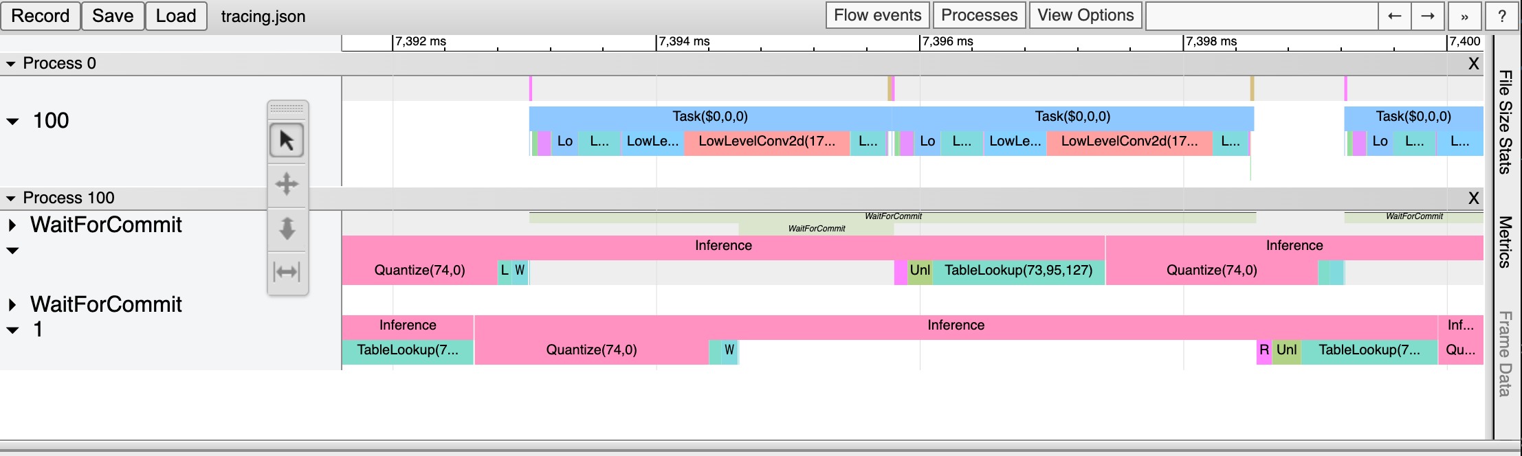
크롬 브라우져에서 주소창에서 chrome://tracing 주소를 입력하면 트레이스 뷰어가
시작된다. 트레이스 뷰어에서 왼쪽 상단에 Load 버튼을 누르고 저장된 파일 (위의 예에서는 tracing.json)
파일을 선택하면 트레이스 결과를 볼 수 있다.
프로파일러 컨텍스트를 이용한 트레이스 생성 활성화
Python 코드에서 프로파일러 컨텍스트(Profiler Context)를 정의하는 것으로도 트레이스 생성을 활성화할 수 있다. 이 방법은 환경 변수를 통한 트레이스 활성화 방법과 비교하여 다음과 같은 장점을 가진다.
Python 인터프리터 또는 Jupyter Notebook와 같은 인터렉티브한 환경에서 바로 트레이스를 활성화 할 수 있다.
실행 구간에 레이블을 붙일 수 있다.
측정을 원하는 연산 카테고리의 선택적으로 측정할 수 있다.
from furiosa.runtime import session, tensor
from furiosa.runtime.profiler import profile

with open("mnist_trace.json", "w") as output:
    with profile(file=output) as profiler:
        with session.create("MNISTnet_uint8_quant_without_softmax.tflite") as sess:
            input_shape = sess.input(0)

            with profiler.record("warm up") as record:
                for _ in range(0, 10):
                    sess.run(tensor.rand(input_shape))

            with profiler.record("trace") as record:
                for _ in range(0, 10):
                    sess.run(tensor.rand(input_shape))
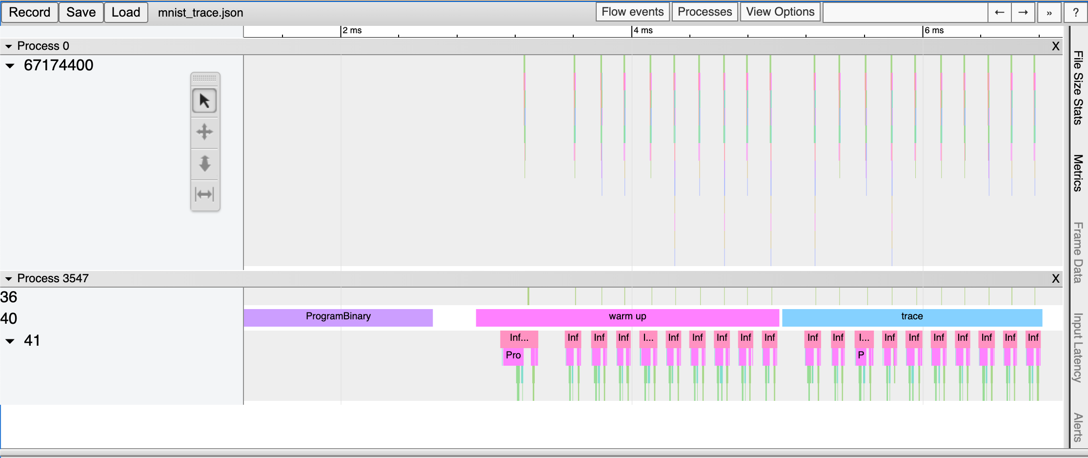
위는 프로파일링 컨텍스트를 활용한 코드 예제이다. 위 Python 코드가 실행되고 나면 mnist_trace.json 파일이 생성되며 트레이스 결과는 아래 그림과 같이 〈warm up’과 〈trace〉 레이블이 붙는다.
Pandas DataFrame을 이용한 트레이스 분석
측정한 트레이싱 데이터를 Chrome Trace Format으로 출력하여 시각화 하는 방법 외에도 데이터 분석에 많이 사용되는 Pandas의 DataFrame으로 표현하고 사용할 수 있다. 이 방법은 Chrome Trace Format과 비교하여 다음과 같은 장점을 가진다.
Python Interpreter 또는 Jupyter Notebook 등의 interactive shell에서 바로 사용할 수 있다.
기본적으로 제공되는 reporting 함수 외에도 사용자가 직접 DataFrame에 접근하여 분석 작업을 수행할 수 있다.
from furiosa.runtime import session, tensor
from furiosa.runtime.profiler import RecordFormat, profile

with profile(format=RecordFormat.PandasDataFrame) as profiler:
    with session.create("MNISTnet_uint8_quant_without_softmax.tflite") as sess:
        input_shape = sess.input(0)

        with profiler.record("warm up") as record:
            for _ in range(0, 2):
                sess.run(tensor.rand(input_shape))

        with profiler.record("trace") as record:
            for _ in range(0, 2):
                sess.run(tensor.rand(input_shape))

profiler.print_summary() # (1)

profiler.print_inferences() # (2)

profiler.print_npu_executions() # (3)

profiler.print_npu_operators() # (4)

profiler.print_external_operators() # (5)

df = profiler.get_pandas_dataframe() # (6)
print(df[df["name"] == "trace"][["trace_id", "name", "thread.id", "dur"]])
위는 프로파일링 컨텍스트의 형식을 PandasDataFrame으로 지정한 코드 예제이다.
(1) 라인이 실행되면 아래와 같이 수행 결과의 요약 정보가 출력된다.
================================================
  Inference Results Summary
================================================
Inference counts                : 4
Min latency (ns)                : 258540
Max latency (ns)                : 650018
Mean latency (ns)               : 386095
Median latency (ns)             : 317912
90.0 percentile latency (ns)    : 564572
95.0 percentile latency (ns)    : 607295
97.0 percentile latency (ns)    : 624384
99.0 percentile latency (ns)    : 641473
99.9 percentile latency (ns)    : 649163
(2) 라인이 실행되면 아래와 같이 하나의 Inference 요청 단위로 소요된 시간 정보가 출력된다.
                            trace_id           span_id  thread.id     dur
40   daf4d8ed300bc4f93901a978111b44f9  d5ac7df24cfd0408         45  650018
81   02e6fb6504e6f7a1312272077a2ca480  313be2a0fb70dc4f         45  365199
124  713e7a122436acbeeafd1339499a7bed  f4402ab5ea873f46         45  258540
173  7e754c14f342d3eb3f4efbc615d15d8a  4f67a754e72e2211         45  270625
(3) 라인이 실행되면 아래와 같이 NPU의 Execution 단위로 소요된 시간 정보가 출력된다.
                          trace_id           span_id  pe_index  execution_index  NPU Total  NPU Run  NPU IoWait
0  e3917c06e01d136ddb98299da74748d8  1b99d7c6574c1c29         0                0      10902     8559        2343
1  a867049bb2db14e62cebe3dc18546923  f5cd3ba0d885fab4         0                0      10901     8557        2344
2  05bfa81f1579ac8089ac75588f36a747  e7e847b44ce11d28         0                0      10997     8557        2440
3  438df7d9beb7fb8c60daaeffbb2c7e76  d2c20e3d9daf21be         0                0      10900     8555        2345
(4) 라인이 실행되면 아래와 같이 Operator 단위로 소요된 시간 정보가 출력된다.
                        average elapsed(ns)  count
name
LowLevelConv2d                   1226.187500     16
LowLevelDepthwiseConv2d           757.333333     12
LowLevelPad                       361.416667     12
LowLevelMask                      116.500000      8
LowLevelExpand                      3.000000      8
LowLevelReshape                     3.000000     68
LowLevelSlice                       3.000000      8
(5) 라인이 실행되면 아래와 같이 CPU에서 동작하는 Operator들에서 소요된 시간 정보가 출력된다.
                            trace_id           span_id  thread.id        name  operator_index    dur
2    daf4d8ed300bc4f93901a978111b44f9  704e2c8ece98e29e         45    Quantize               0  42929
3    daf4d8ed300bc4f93901a978111b44f9  4a304c8c46be707a         45       Lower               1  72999
34   daf4d8ed300bc4f93901a978111b44f9  cff0f3268f26423d         45     Unlower               2  31812
36   daf4d8ed300bc4f93901a978111b44f9  b3a90233e6eb90f8         45  Dequantize               3   4895
54   02e6fb6504e6f7a1312272077a2ca480  920c7170893cb202         45    Quantize               0  14085
55   02e6fb6504e6f7a1312272077a2ca480  b2508624adaf01a1         45       Lower               1  32360
75   02e6fb6504e6f7a1312272077a2ca480  ed6fc23c0a7cc81e         45     Unlower               2  15655
78   02e6fb6504e6f7a1312272077a2ca480  e2d61265a1fe0ad6         45  Dequantize               3   6128
96   713e7a122436acbeeafd1339499a7bed  20473c3a26d91593         45    Quantize               0   4400
100  713e7a122436acbeeafd1339499a7bed  f71676c0868f1a34         45       Lower               1  28714
118  713e7a122436acbeeafd1339499a7bed  dff936584542ee83         45     Unlower               2  12675
121  713e7a122436acbeeafd1339499a7bed  9d2eaf76f1a6d156         45  Dequantize               3  12227
138  7e754c14f342d3eb3f4efbc615d15d8a  0df3b383e59e5322         45    Quantize               0   6631
142  7e754c14f342d3eb3f4efbc615d15d8a  c15504b489f56503         45       Lower               1  11694
170  7e754c14f342d3eb3f4efbc615d15d8a  cb8f9199904c6065         45     Unlower               2  17573
171  7e754c14f342d3eb3f4efbc615d15d8a  90c1af4de00eebc2         45  Dequantize               3  16021
(6) 라인을 실행하면 코드에서 DataFrame에 접근하고 사용자가 직접 분석할 수 있다.
                            trace_id   name  thread.id     dur
150  ec3dd3d28baf03adc6a1ddd5efe319bc  trace         44  778887