Reducer
The Reducer performs elementwise multiplication followed by reduce-add. Each slice’s Reducer contains 8 independent Rows, which are parallel MAC lanes that each process a different weight channel. It receives input data from the Stream Adapter and weight data from the TRF Sequencer.
Interface
The Reducer is invoked via .align() followed by .contract() and .accumulate():
extern crate furiosa_visa_std;
use furiosa_visa_std::prelude::*;
impl CollectTensor<'l, T, D, Chip, Cluster, Slice, Time, Packet> {
    /// Aligns input stream and TRF to computation mapping.
    pub fn align<OutTime: M, OutPacket: M, Row: M, TrfElement: M>(
        self,
        trf: &TrfTensor<D, Chip, Cluster, Slice, Row, TrfElement>,
    ) -> AlignedPair<'l, T, D, Chip, Cluster, Slice, Row, OutTime, OutPacket>;
}

impl AlignedPair<'l, T, D, Chip, Cluster, Slice, Row, Time, Packet> {
    /// Performs spatial reduction: elementwise multiplication followed by reduce-add
    /// across the Packet dimension via the hardware reduction tree.
    /// Data type is widened during contraction: i4/i8 -> i32, f8/bf16 -> f32.
    pub fn contract<OutPacket: M>(
        self,
    ) -> ContractionTensor<'l, T, OutD, Chip, Cluster, Slice, Row, Time, OutPacket>;
}

impl ContractionTensor<'l, T, D, Chip, Cluster, Slice, Row, Time, Packet> {
    /// Performs temporal accumulation: accumulates values over the Time dimension
    /// and produces the final contraction output.
    pub fn accumulate<OutTime: M, OutPacket: M>(
        self, kind: AccumulationKind,
    ) -> AccumulationTensor<'l, T, D, Chip, Cluster, Slice, OutTime, OutPacket>;
}
The Reducer computes the dot product of input stream \(X\) and TRF weights \(W\):
$$\text{output}[i] = \sum_{j} X[i, j] \times W[i, j]$$
The summation index \(j\) corresponds to axes removed during reduction:
- Spatial reduction removes axes from the
Packetdimension via the hardware reduction tree - Temporal reduction removes axes from the
Timedimension via the accumulator buffer
The output mapping is determined by which axes survive reduction: OutPacket contains Packet axes after spatial reduction, and OutTime contains Time axes after temporal reduction.
Examples
Matrix Multiplication
Matrix multiplication with 8 Rows operating in parallel:
#![allow(unused)]
fn main() {
#![feature(adt_const_params)]
extern crate furiosa_visa_std;
use furiosa_visa_std::prelude::*;
axes![A = 32, B = 32, C = 8];

fn matmul<'l, const T: Tu>(
    input: CollectTensor<'l, T, bf16, m![1], m![1], m![1], m![A, B / 16], m![B % 16]>,
    trf: &TrfTensor<bf16, m![1], m![1], m![1], m![C], m![B]>,
) -> AccumulationTensor<'l, T, f32, m![1], m![1], m![1], m![A], m![C]> {
    // Computation mapping: [
    //   Time: [A = 32],
    //   Row: [C = 8],
    //   Packet: [B = 32] (32 bf16 elements = 64 bytes)
    // ]
    //
    // Spatial reduction: tree depth 5 reduces 32 bf16 elements along B → f32
    // Output (Interleaved): Time = [A], Packet = [C]
    input.align::<m![A], m![B], _, _>(&trf)
         .contract::<m![1]>()
         .accumulate::<m![A], m![C]>(AccumulationKind::Interleaved)
}
}
At each Row, elementwise multiplication of input * trf occurs.
With tree depth 5, reduce-add sums over the 32 bf16 elements of B, producing one f32 per A position.
Full Tensor Reduction
This example demonstrates a complete reduce-add over a tensor m![A] with m![A]::SIZE = 65536, showing how spatial and temporal reduction combine with slice-level reduction.
Mapping:
Slice = mTime = mPacket = m
Reduction breakdown:
| Stage | Axes Reduced | Mechanism | Cycles |
|---|---|---|---|
| Spatial | A % 32 | Reducer tree (depth 5) | 5 |
| Temporal | A / 32 % 8 | Reducer accumulator (8 iterations) | 8 |
| Slice-level | A / 256 | Inter-Slice Block | 256 |
Analysis:
- Each slice processes
A / 256(256) elements - Within a slice:
A % 32elements are reduced spatially by the tree (5 cycles forbf16) - The temporal axis
A / 32 % 8means 8 flits arrive sequentially, accumulated by the buffer - After in-slice reduction completes (~40 cycles), 256 partial results exist across slices
- The Inter-Slice Block reduces these 256 slice results (256 cycles)
- Total: ~296 cycles for reducing 65536 elements to a single scalar
Architecture
The Reducer consists of 8 independent Rows operating in parallel. Data flows to the Rows from two sources:
- StreamUnit data: Broadcast to all Rows (same data to every row)
- TRF data: Read in parallel from 8 independent Row spaces (TRF Row \(i\) feeds Row \(i\) directly)
Each Row contains a reduction tree for spatial reduction, followed by a shared accumulator buffer for temporal reduction.
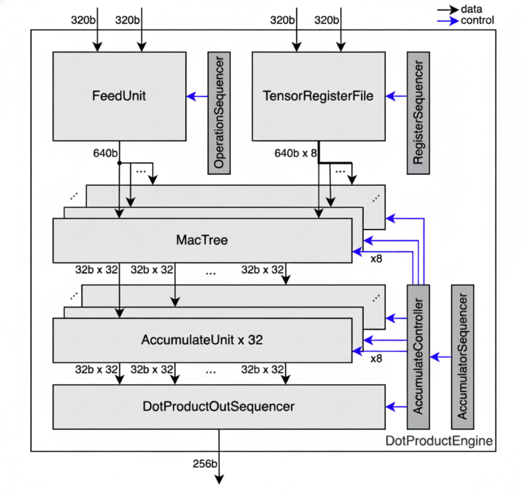
The diagram shows data widths at different stages. The 320b/640b corresponds to 64/128 elements for i4/i5, 32/64 elements for i8/f8/i9, 16/32 elements for bf16, and 8/16 elements for f32/i32.
Spatial Reduction
Each Row contains a reduction tree that sums products hierarchically.
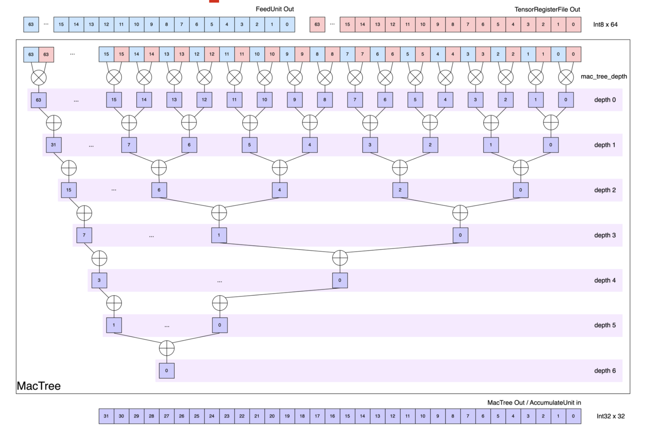
At depth 0, each Row multiplies the input stream from the Stream Adapter, with the weight data from the TRF Sequencer (each 64 bytes wide). Each subsequent depth sums pairs of partial products, halving the element count from the previous depth. The tree depth varies by data type to provide sufficient depth for reducing the full data width:
i4: depth 7 (reduces 128 elements)i8/f8: depth 6 (reduces 64 elements)bf16: depth 5 (reduces 32 elements)
The output data type is widened to accommodate larger result values from contraction.
With i8 input, i8 * i8 multiplication occurs first, and up to 64 values can be summed across the 6-depth tree.
Inputs i4/i8 produce i32 outputs, and inputs f8/bf16 produce f32 outputs.
Given a computation mapping of m![Row, Time, Packet], spatial reduction eliminates the innermost m![Packet % 2^n] axes (where n is the tree depth), producing an output mapping of m![Row, Time, Packet / 2^n].
Note
Spatial reduction in
additionmode allows full 8-Row usage, butmaxmode only supports a single Row (Row 0).
Resize
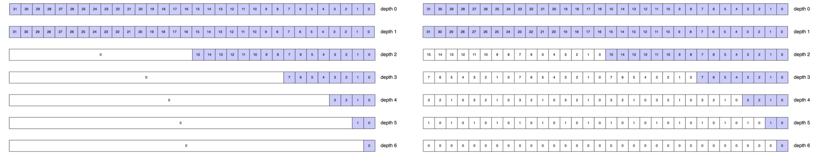
After spatial reduction, the output is resized to exactly 32 i32/f32 elements per Row before being fed to the temporal accumulator.
When the tree depth is 0 (no spatial reduction), the 32 outer elements are truncated.
Otherwise, the spatial reduction output is padded or broadcast to fill the 32 columns of the temporal accumulator, depending on the output mode.
The Reducer supports two output modes that determine how the resize is performed:
- Sequential: Rows are sequentially ordered. The spatial reduction output is padded with zeros.
- Interleaved: Rows are interleaved. The spatial reduction output is repeated across the 32 columns.
The figure below illustrates the output of spatial reduction for various i8 reduction depths.
The left side shows Sequential mode adding zero-padding; the right shows Interleaved mode replicating the output to fill 32 element positions.
Temporal Reduction
After resizing, each Row feeds its output to a shared temporal accumulator.
The temporal accumulator stores intermediate results in a buffer and accumulates values that arrive sequentially over time, enabling reduce operations even when the reduce axis is not contiguous in the innermost dimension.
The buffer has 1024 slots total: 8 rows × 32 columns × 4 registers/column.
Consider axes![A = 2048, B = 8] and a tensor with mapping m![A, B], where we want to reduce along axis B.
With mapping Time = m![B / 4, A % 8] and Packet = m![B % 4], the spatial reduction stage outputs 16 flits (since Time::SIZE = m![B / 4, A % 8]::SIZE = 2 * 8 = 16).
The accumulator uses 8 buffer slots (one per A % 8 value) to accumulate across the B / 4 (2) iterations:
| flit # | B / 4 | A % 8 | Buffer Slot | Operation |
|---|---|---|---|---|
| 0 | 0 | 0 | 0 | Store |
| 1 | 0 | 1 | 1 | Store |
| 2 | 0 | 2 | 2 | Store |
| 3 | 0 | 3 | 3 | Store |
| 4 | 0 | 4 | 4 | Store |
| 5 | 0 | 5 | 5 | Store |
| 6 | 0 | 6 | 6 | Store |
| 7 | 0 | 7 | 7 | Store |
| 8 | 1 | 0 | 0 | Accumulate with flit #0 |
| 9 | 1 | 1 | 1 | Accumulate with flit #1 |
| 10 | 1 | 2 | 2 | Accumulate with flit #2 |
| 11 | 1 | 3 | 3 | Accumulate with flit #3 |
| 12 | 1 | 4 | 4 | Accumulate with flit #4 |
| 13 | 1 | 5 | 5 | Accumulate with flit #5 |
| 14 | 1 | 6 | 6 | Accumulate with flit #6 |
| 15 | 1 | 7 | 7 | Accumulate with flit #7, then output |
The first 8 flits are stored in buffer slots 0-7. When flits 8-15 arrive, they accumulate with the stored values. After flit 15, the buffer contains the final reduced results and outputs them.
For buffered reduction to work, the product of all axis sizes inner to the reduce axis must be at most 1024, in order to fit the accumulator buffer.
The temporal accumulator supports two operation modes: Sequential and Interleaved.
Interleaved provides a greater buffer capacity of 128 for the axes inner to the reduce axis, compared to the Sequential 32-element capacity. However, Interleaved changes the output packet structure. Choose the mode based on buffer constraints and whether the desired output ordering matches downstream requirements. See Constraints for the full buffer capacity rules.
Interleaved Mode
In Interleaved mode, the Reducer outputs data element-by-element across all Rows. The output bus carries one value from each of the 8 Rows, per beat.
- Packet Slicing: In Interleaved mode, not all of
Packetis fed to the accumulator. Since the reduction tree broadcasts \(m\) partial sums across all 32 column positions (via replication), only the first \(m\) columns get written to accumulator entries, slicingPacketfrom 32 down to \(m\).
Note
User-specified slicing should only slice padded
Packetaxes.
-
Column Interleaving: To achieve maximum accumulator utilization, all of the 32 accumulator columns are filled by interleaving \(\frac{32}{m}\) column groups over successive cycles. For \(m = 4\), the first cycle writes to columns 0–3, the next to columns 4–7, and so on, giving 8 interleave steps to fill all 32 columns.
-
Full Row Utilization: Additionally, all 8 accumulator rows are always active regardless of the actual input Row count: if
Row < 8, the data is padded to occupy all 8 Rows. -
Output:
OutTime: m![Time', Packet / 2^n = m],OutPacket: m![Row # 8].OutTimepreserves the order ofTime, Packet, but with some axes fromTimeremoved. The removed axes undergo reduce-add, yieldingTime'.OutPacketequalsRowpadded with dummies to align to 8, as all Rows are utilized.
Note
Interleavedmode has reduced accumulator utilization whenRow< 8: onlyRowout of 8 rows store meaningful data, while the output bus always sends all 8 Rows together. Effective accumulator capacity isRow× 32 × 4 instead of the full 8 × 32 × 4 = 1024 slots. This limitation is most severe atRow = 1(128 useful slots), but applies toRow = 2andRow = 4as well.
Example
This example performs a contraction where K is partially reduced spatially (K % 4 in Packet) and temporally (K / 16 in Time), with K % 16 / 4 surviving in the output:
#![allow(unused)]
fn main() {
#![feature(adt_const_params)]
extern crate furiosa_visa_std;
use furiosa_visa_std::prelude::*;
axes![M = 4, N = 8, K = 64];

fn interleaved<'l, const T: Tu>(
    input: CollectTensor<'l, T, bf16, m![1], m![1], m![1], m![K / 16, M], m![K % 16]>,
    trf: &TrfTensor<bf16, m![1], m![1], m![1], m![N], m![K]>,
) -> AccumulationTensor<'l, T, f32, m![1], m![1], m![1], m![M, K % 16 / 4], m![N]> {
    // Computation mapping:
    //   Time: [K / 16, M], Row: [N], Packet: [K % 16]
    //   16 bf16 elements per packet = 32 bytes
    //
    // Spatial: tree depth 2 reduces groups of 4 bf16 -> 1 f32,
    //          leaving K % 16 / 4 (4) columns
    // Temporal: K / 16 (4) iterations accumulated in buffer
    //
    // Interleaved output:
    //   m = 4 valid columns, 16 / 4 = 4 column groups interleaved
    //   OutTime = [M, K % 16 / 4] (K / 16 reduced, surviving Packet appended)
    //   OutPacket = [N] (Row, already 8)
    input.align::<m![K / 16, M], m![K % 16 # 32], _, _>(&trf)
         .contract::<m![K % 16 / 4]>()
         .accumulate::<m![M, K % 16 / 4], m![N]>(AccumulationKind::Interleaved)
}
}
The axes inner to the reduce axis (K / 16) are M and K % 16 / 4, with a total size of 4 × 4 = 16.
This satisfies the Interleaved buffer constraint (≤ 128).
Sequential Mode
In Sequential mode, the Reducer outputs the reduced data in each Row sequentially.
The output bus carries up to 8 elements from Packet, per beat.
-
Full Packet Utilization: In Sequential mode, all 32 columns of
Packet / 2^nare fed to the accumulator. Unlike in Interleaved mode, no packet slicing occurs. Each cycle writes all 32 columns simultaneously, with zeros padding any unused positions. -
Row Interleaving: To achieve maximum accumulator utilization, all 8 accumulator rows are filled by interleaving \(\frac{8}{\texttt{Row}}\) row groups over successive cycles. With
Row::SIZE = 4, the first 4 rows of the temporal accumulator store rows 0–3, and, in the next cycle, the next 4 rows store in rows 4–7. -
Output:
OutTime: m![Time', Row, Packet_outer],OutPacket: m![Packet_inner].OutTimepreserves the order ofTime, Row, but with some axes fromTimeremoved. The removed axes undergo reduce-add, yieldingTime'.- Since the output bus is 8 elements-wide, only multiples of 8 elements (8, 16, 24, or 32) can be output.
Packetis split accordingly:Packet_outer = m andPacket_inner = m.
Example
The same computation mapping as the Interleaved example above, but with Sequential output:
#![allow(unused)]
fn main() {
#![feature(adt_const_params)]
extern crate furiosa_visa_std;
use furiosa_visa_std::prelude::*;
axes![M = 4, N = 8, K = 64];

fn sequential<'l, const T: Tu>(
    input: CollectTensor<'l, T, bf16, m![1], m![1], m![1], m![K / 16, M], m![K % 16]>,
    trf: &TrfTensor<bf16, m![1], m![1], m![1], m![N], m![K]>,
) -> AccumulationTensor<'l, T, f32, m![1], m![1], m![1], m![M, N], m![K % 16 / 4 # 8]> {
    // Computation mapping:
    //   Time: [K / 16, M], Row: [N], Packet: [K % 16]
    //   16 bf16 elements per packet = 32 bytes
    //
    // Spatial: tree depth 2 reduces groups of 4 bf16 -> 1 f32,
    //          leaving K % 16 / 4 (4) columns
    // Temporal: K / 16 (4) iterations accumulated in buffer
    //
    // Sequential output:
    //   Packet'' = K % 16 / 4, padded to 8:
    //     - Packet_outer = [1],
    //     - Packet_inner = [K % 16 / 4 # 8]
    //   OutTime = [M, N] (K / 16 reduced, Row appended)
    //   OutPacket = [K % 16 / 4 # 8] (surviving Packet padded to 8)
    input.align::<m![K / 16, M], m![K % 16 # 32], _, _>(&trf)
         .contract::<m![K % 16 / 4]>()
         .accumulate::<m![M, N], m![K % 16 / 4 # 8]>(AccumulationKind::Sequential)
}
}
The axes inner to the reduce axis (K / 16) are M and N, with a total size of 4 × 8 = 32.
This satisfies the Sequential buffer constraint (≤ 32).
Note
Sequentialmode has reduced accumulator utilization whenPacketis spatially reduced: onlyPacket / 2^nout of 32 elements store meaningful data per Row. Effective accumulator capacity is 8 × 1 × 4 = 32 slots instead of the full 1024. This limitation applies whenever the non-padded portion ofPacket / 2^nis fewer than 32 elements.
Constraints
- Row count: The hardware provides exactly 8 Rows. Operations can use 1, 2, 4, or 8 rows, but the
Rowdimension size must match one of these values. - Tree depth: Determines how many elements can be reduced spatially. Depth 7 for
i4(128 elements), depth 6 fori8/f8(64 elements), depth 5 forbf16(32 elements). The input packet size must not exceed the maximum elements reducible at the given depth. - Spatial output limit: For a tree depth of 0 (no spatial reduction), the Reducer outputs at most 32
i32/f32elements. Configurations that would produce more than 32 output elements per cycle are invalid. - Data types: Input types must be
i4,i8,f8, orbf16. Output types are automatically widened toi32(fromi4/i8) orf32(fromf8/bf16). The type widening is mandatory. - Reduce-max: Only supports using a single Row (Row 0), limiting reduce-max throughput to 1/8th of reduce-add capacity.
- Buffer capacity: The accumulator has 1024 buffer slots (8 rows × 32 columns × 4 registers/column). The product of axes inner to the outermost reduce axis must fit within this capacity.
- Interleaved constraints: Requires axes inner to outermost reduce in
OutTimeto be at most 128. Full constraint:align_up(Row, 8) * (axes inner to reduce)≤ 1024. - Interleaved utilization: When
Row< 8, effective capacity is reduced toRow× 32 × 4 slots, preventing full buffer utilization. - Sequential constraints: Requires axes inner to outermost reduce in
OutTimeto be at most 32. Full constraint:align_up(reduced_packet.len(), 32) * (axes inner to reduce)≤ 1024. - Sequential utilization: When
Packetis reduced, full buffer utilization cannot be achieved. For instance, when reducingPackettotally, only one column of each Row is used, wasting 31/32 of the buffer capacity.
- Interleaved constraints: Requires axes inner to outermost reduce in
Performance
- Spatial latency: Tree depth determines spatial reduction latency:
i4depth 7 (128 elements in 7 cycles),i8/f8depth 6 (64 elements in 6 cycles),bf16depth 5 (32 elements in 5 cycles). Shallower trees complete faster, but larger data types require less depth due to narrower data paths. - Temporal latency: Each accumulation cycle processes one packet. For a reduction axis of size
Nin the time dimension, the accumulator requires approximatelyNcycles to complete the reduction. - Parallelism: Using all 8 Rows maximizes throughput. Each Row operates independently, so 8 rows achieve 8× parallelism compared to a single row.
- Type widening: Output data types are widened to prevent overflow (
i4/i8→i32,f8/bf16→f32). This widening is automatic and adds minimal latency, but downstream components must handle 32-bit data. - Reduce-max: Only supports single Row (Row 0) usage, limiting parallelism to 1/8th of reduce-add throughput.
- Truncation: When tree depth is 0, the Reducer can output at most 32 elements spatially. Larger packets are truncated.
- Pipeline integration: The Reducer sits between Stream Adapter/TRF Sequencer and Vector Engine, adding latency proportional to tree depth plus time dimension size.